Introduction

DELPHI (DNA Explorer for Locus-based Population History Insights) is a web-based genome browser designed for exploring population genetics in modern and ancient humans. DELPHI computes population genetic statistics on-the-fly based on your selections, giving you flexibility to compare populations and explore genetic variation across the human genome. The server comes preloaded with ancient genomes from the Allen Ancient DNA Resource (AADR), modern genomes from gnomAD v3.1.12 (harmonised HGDP and the 1000 Genomes Project database). Samples are aligned to the hg38 reference genome.

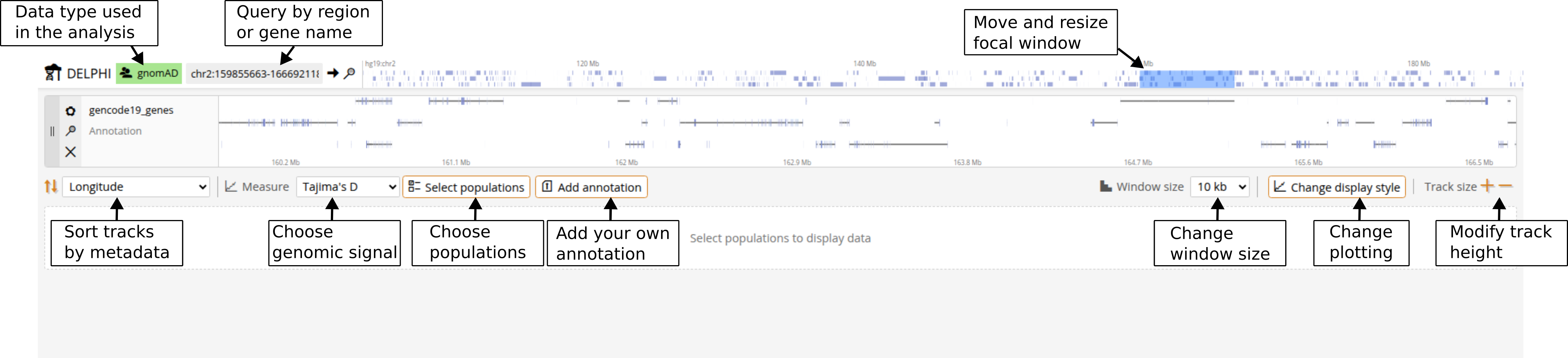
Navigation is similar to other genome browsers. To jump to a specific location, type coordinates in the query box at the top (e.g., chr1:5000000-7000000). You can zoom in and out using Ctrl+scroll on any track, or by double-clicking on a region of interest. The visible annotation region is determined by the blue rectangle at the top. You can resize and drag it to adjust the window you want to examine. You can also click and drag the annotation track to pan left or right. As you drag, all tracks update together.

Selecting populations

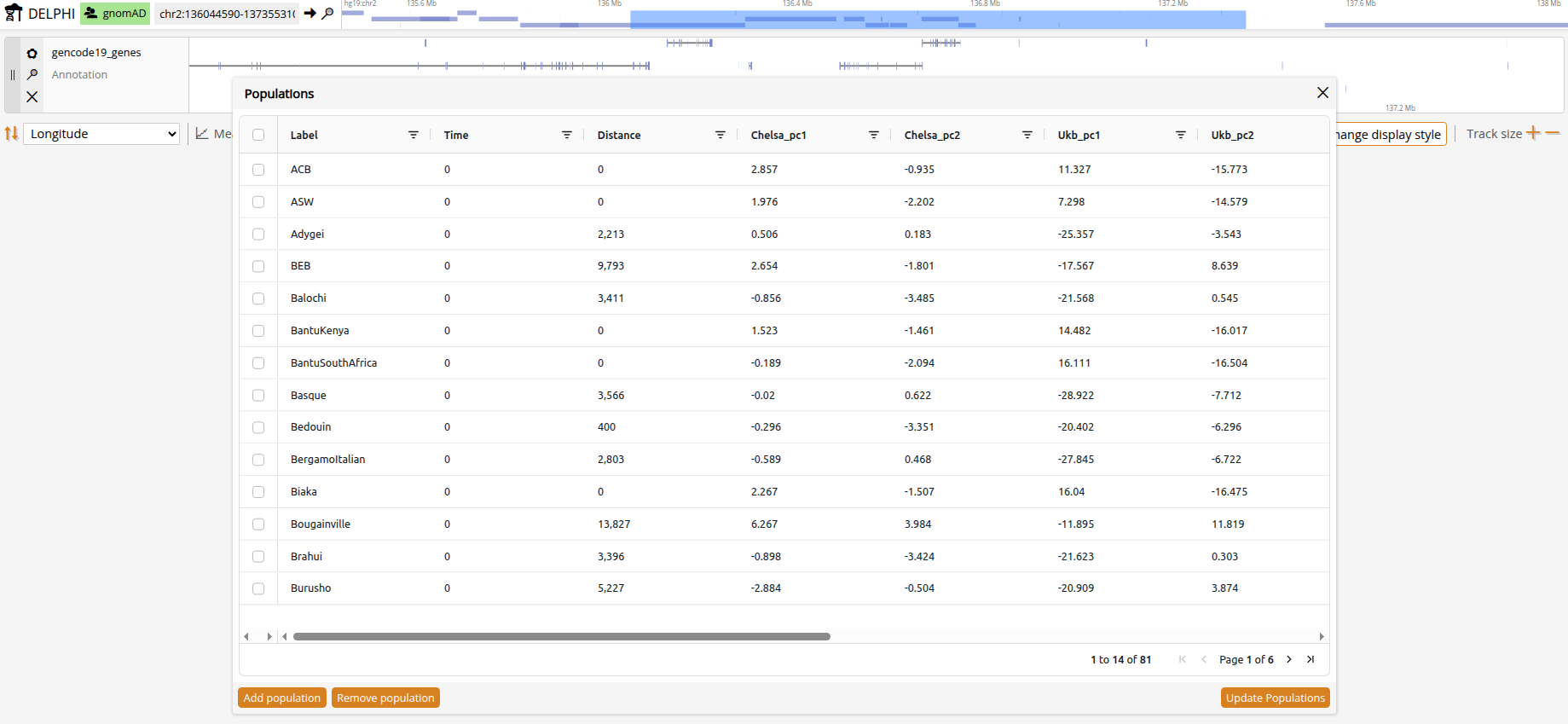
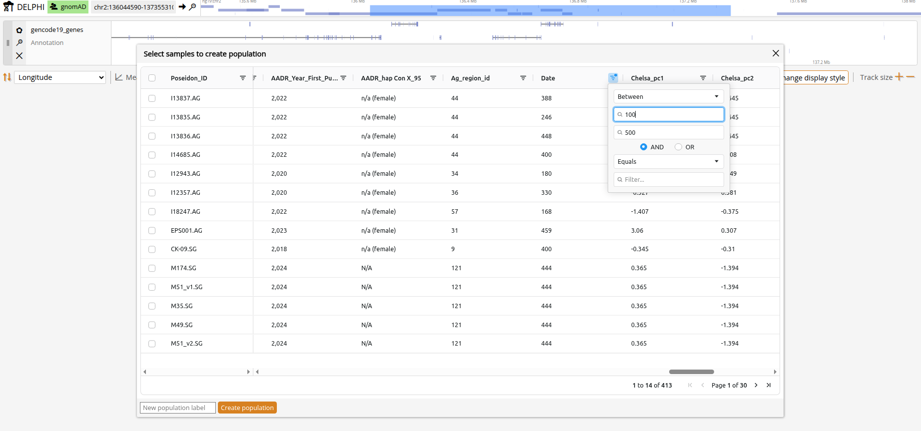
Click the Populations button in the top navigation bar to open the population selector. The population list shows all available populations with their metadata. Becuase there are currently no established clustering methods designed for aDNA, predefined ancient populations were simply clustered by time and geography and are provided mainly to get you started without a background in ancient DNA. To gain full flexibilty, you can click on "Add population" and define custom populations based on sample IDs or metadata filters. For example, you can group all female samples younger than 500 by marking in the 'Genetic_Sex' column 'contains==F' and in the 'Date' column 'less than==500'. After you click "Create population" you will see your new population in the main population selection pop-under Dataset==USER. Click "Update populations" when finished.

Metadata

Samples and populations in DELPHI have rich metadata information. You can use it to define populations and sort the population signal tracks. Population-level metadata is computed for the median of samples. The metadata include:

• Geographic coordinates (latitude and longitude ranges)
• Waypoint distance (distance by migratory routes, excluding large bodies of water)
• Date (0 for modern samples)
• Climate variables from CHELSA-TraCE21k, a high-resolution climate data set for the global land surface area covering both modern and historical bioclimatic layers. We use a PCA-based summary data with PC1 reflects temperature-related variation and PC2 primarily reflects precipitation-related variation.
• Genetic similarity. Based on UKBiobank PCA distance.
• Sociocultural transitions. The onset of the Neolithic Revolution and the rise of urbanized societies. Taken from the ArchaeoGLOBE database.

Genomic signals

Choose what genetic signal to visualize using the Measure dropdown below the annotation track. Most measures are computed per-SNP and returned in non-overlapping bins of minimum 10kb (per-SNP plots become visually cluttered and noisy). To control the resolution, you can choose the window size of the plots. The larger the window, the smoother the signal.

Per-population signals

Heterozygosity

Expected heterozygosity measures the genetic diversity within a population by quantifying the probability that two randomly chosen alleles at a locus differ from each other. Higher heterozygosity indicates greater genetic diversity. DELPHI computes expected heterozygosity as 2pq, where p is the allele frequency and q = 1-p, calculated separately for each SNP. Allele counts (AC) and allele numbers (AN) are derived from the genotype data for each population, accounting for missing data. The per-SNP heterozygosity values are then aggregated into windows using the mean value across all variants in each window.

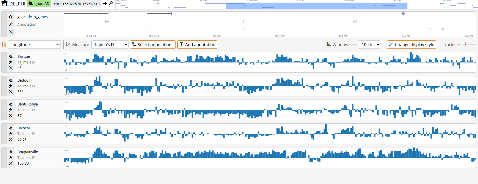
Tajima's D

Tajima's D is a statistical test that compares the average number of pairwise differences between sequences to the number of segregating sites. It is used to detect deviations from neutral evolution. Negative values suggest an excess of rare alleles (population expansion or purifying selection), while positive values indicate an excess of intermediate-frequency alleles (balancing selection or population contraction). DELPHI computes Tajima's D using standard population genetic formulas, comparing observed genetic diversity patterns to neutral expectations.

Fu and Li's F*

Fu and Li’s F* is a site-frequency-spectrum neutrality test that contrasts nucleotide diversity (π) with the number of singleton variants (η_s) among segregating sites (S). Because ancestral states are not required, DELPHI computes the no-outgroup version (F*) using minor-allele singletons. Negative values indicate an excess of singletons relative to π (often consistent with recent population expansion or purifying/background selection), whereas positive values indicate a deficit of singletons (e.g., population contraction or balancing selection). DELPHI derives allele counts and allele numbers per SNP from the genotype data (accounting for missingness), defines singletons as variants with minor allele count = 1, and computes F* from window-level aggregates; windows with fewer than 3 segregating sites return missing values.

Pairwise signals

FST

Fst measures genetic differentiation between populations by quantifying the proportion of total genetic variance that is due to population structure. Values range from 0 (no differentiation) to 1 (complete differentiation). Higher Fst values indicate greater genetic distance between populations. DELPHI computes Fst per-SNP using Weir and Cockerham's method, which accounts for differences in sample sizes and provides unbiased estimates. Allele frequencies are calculated for each population from the genotype data, and Fst is computed by comparing the variance in allele frequencies between populations relative to the total variance. Values are then aggregated into windows by averaging across SNPs.

With multiple populations selected, you will have multiple data tracks displayed simultaneously. By default, tracks appear alphabetically. To identify potential explanatory variables, you can sort tracks based on various metadata. Once you've identified regions of interest, click the Export button to download your current view as a tabular file (CSV format). The export includes genomic coordinates, measure values for each population or population pair, and population labels. You can then perform statistical tests, make publication-quality plots, or integrate with other data in your downstream analysis pipeline.

Adding annotations

Click the Add annotation button to load a custom annotation track in GFF or GTF format. These files store genomic features as intervals with attributes, and can represent, for example, transposable elements/repeats, promoters/enhancers, non-coding RNAs, CpG islands/UTRs, variant or CNV intervals, conserved elements, or experimental peak tracks (e.g., ChIP-seq). Uploaded tracks appear below the default annotation tracks and are rendered automatically while you navigate and zoom, helping you interpret population-genetic signals in the context of specific genomic features.